SWE-GNN

Summary

• Bentivoglio et al. (2023) implements GNN in modeling dyke breach flooding in synthetic randomly generated conditions.
• Domain is relatively smaller.
• Proposed model works well.
• Application to raifall, storm surge, discharge generated flood remains as future work.

Background/Problem statement

• Numerical modeling is accurate but computationally expensive
• Previously neural networks are used for surrogate modeling
• Most models are case specific , with limited generalizability and time-dependent applications. Point out that most models are trained for a particualar area, and to apply it to other areas, retraining is needed.
• Some studies that attempt to generalize over unseen area typically focues on single maximum depth or velocity map without considering temporal dynamics.
• Shallow water equation graph neural network (SWE-GNN) is proposed for rapid spatio-temporal flood modeling to address the above issues.

Theoretical background

• Shallow Water Equations: a system of hyperbolic partial differential equations that describle shallow water flows by enforcing mass and momentum conservation
  • Mostly 2D SWE is used for flood modeling
• Finite Volume Method: spatio-temporal numerical discretizations
• Deep learning:
  • Most common type is MLP, but they are non-inductive. Model trained on one condition cannot be applied to completely different condition
  • GNN upto some extent address non-inductive issue.
  • Standard GNN do not include physics-based propagation rules.

SWE inspired GNN

• Architecture: Encoder-processor-decoder

$$U^{t+1}=U^t+\varphi (X_s,U^{t-p:t},E)$$

• Encoder

  • Three separate encodes for static, dynamic and edge features
  • 2 MLPs layers with parametric ReLU activation, hidden dimension G
  • Expand the dimensionality of inputs to allow for higher expressibity

• Processor

  • L-layer GNN that takes encoded inputs features
  • Propagation rules based on SWE

  

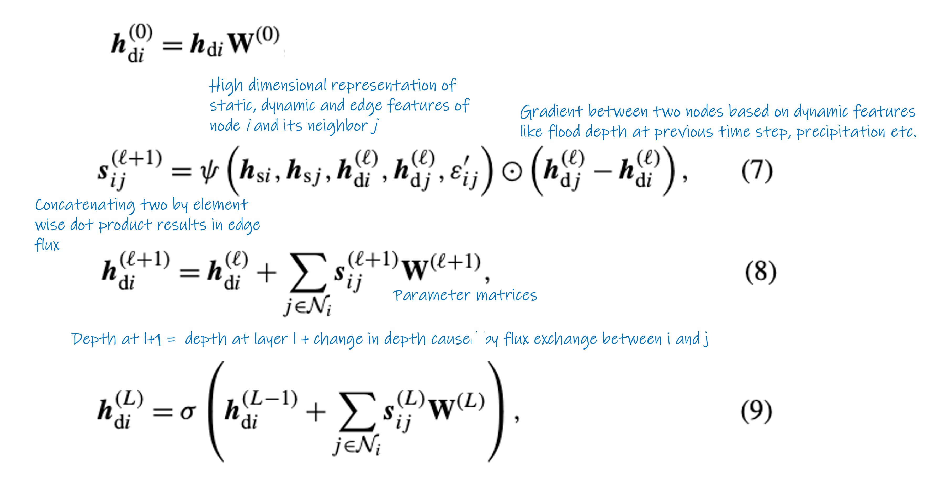
• Decoder

  • One MLP (2-layers, PReLU, G) shared across all nodes, that takes output from processor layer as input
  • Predict hydraulic variable at next time step
  • No bias term in MLPs in the dynamic encoder and the decoder because adding bias term would result non-zero values to dry nodes

• 8 GNN layers, with G = 64

Inputs and outputs

• Static node features: area of cell, elevation, slope, manning coefficient and water level at time step t
  • why $w_i^t$ on static?
• Dynamic node features: flood depth ($h_i^t$) and unit discharge ($|q{|}_i^t$)
• Edge features: outward unit normal vector ($n_{ij}$) and cell sides’ length ($l_{ij}$)
• Outputs: Water depth and unit discharge at time $t+1$

Training strategy

• Multi-step-ahead loss function that measure accumulated error over consecutive time steps (K-step rollout)
• Curriculum learning strategy: first learn one-step ahead and then to increase number of steps ahead to stablize the predictions
• Adam Optimization
• Starting LR = 0.005, fixed step decay of 90% every 7 epochs
• Trained for 150 epochs

Datasets

• Dataset generation: 130 numerical simulations of dike breach floods

  • randomly generated topographies using Perlin Noise Generator
  • 2 domains 6.4 x 6.4 and 12.8 x 12.8 $k{m}^2$
  • Delft3D-FM used to solve full SWE
  • Dry bed as initial condition
  • Constant input discharge of 50 $m^3/s$ as boundary condition
  • Simulation output is flood maps at 30 min time steps

• Three datasets:

  1. First
  • 100 DEMs over 64 x 64 grid
  • dx = 100 m
  • Simulation period = 48 h
  2. Second
  • 20 DEMs over 64 x 64 grid
  • dx = 100 m
  • Simulation period = 48 h
  • Change in breach location. To test generalizability of the model to unseen domains and breach locations
  3. Third
  • 10 DEMs over 128 x 128 grid
  • dx = 100 m,120h
  • To test generalizability of the model to large unseen domains

• Temporal resolution of ML model: 1 h

Performance

• RMSE
  • h: $0.11\pm 0.051$ m
• MAE
  • h: $0.004\pm 0.001$ m
• CSI
  • $\tau =0.05m$
    • $75.85\pm 9.30$
  • $\tau =0.3m$
    • $73.44\pm 9.28$

Note

MAE and RMSE increase over time due to the evaluation of both metrics via a spatial average, which implies that, in the first time steps, where the domain is mostly dry, the error will naturally be lower.

Finding

GNN valuable tool for spatio-temporal surrogate modelling of floods.

Limitations

• Constant boundary condition. In reality, boundary condition varies with time. In case of compound flood modeling we need to consider time varying boundary condition.

This work is further extended to Multi-scale SWE GNN.